Getting Started with the didet Package

Introduction

The didet package provides tools for differences-in-differences (DiD) estimation when the treatment variable of interest may be non-binary and its value may change in each time period. The package implements the doubly robust estimation of the average treatment effect for movers using the concept of effective treatment. The methods are developed by Yanagi (2023) “An effective treatment approach to difference-in-differences with general treatment patterns”.

Installation

Get the package from GitHub:

# install.packages("devtools") # if necessary
devtools::install_github("tkhdyanagi/didet", build_vignettes = TRUE)

Package Function

The didet package provides the following function:

didet(): DiD estimation with general treatment patterns using the concept of effective treatment.

Arguments

The didet() function has the following arguments:

yname: The name of the outcome variable
dname: The name of the treatment variable
tname: The name of the time period
idname: The name of the unit index
xformla: A formula for the unit-specific covariates to be included. It should be of the form xformla = ~ X + Z. Default is xformla = ~ 1.
data: A data.frame of balanced panel data (long format)
specification: A character specifying the effective treatment function. Options are “once”, “event”, “number”, and “aggregate”. Default is “event”.
alp: The significance level. Default is 0.05.
nboot: The number of bootstrap repetitions. Default is 1000.

Returns

The didet() function returns a list that contains the following elements:

ATEM: A data.frame that collects the estimation results for \(\mathrm{ATEM}(t, s, e)\) and \(\mathrm{ATEM}(t, s, r, e)\).
mover: A data.frame that collects the estimation results for the probabilities of being movers.
stayer: A data.frame that collects the estimation results for the probabilities of being stayers.
figure: A list that contains the ggplot2 figures for \(\mathrm{ATEM}(t,s,e)\) and \(\mathrm{ATEM}(t, s, r, e)\).

Example

We begin by generating artificial balanced panel data using the datageneration() function.

# Generate artificial balanced panel data
# N: The number of the cross-sectional units
# S: The length of the time series
set.seed(1)
data <- didet::datageneration(N = 1000, S = 4)
head(data)
#>   id period          Y D          X once event number
#> 1  1      1 -0.1819699 0 -0.6264538    0     0      0
#> 2  1      2  2.2096505 1 -0.6264538    1     2      1
#> 3  1      3  1.4318668 0 -0.6264538    1     2      1
#> 4  1      4  2.8392303 1 -0.6264538    1     2      2
#> 5  2      1 -0.6832054 0  0.1836433    0     0      0
#> 6  2      2  4.9496969 0  0.1836433    0     0      0

The event specification

The DiD estimation using the event specification:

# DiD estimation
did_est <- didet::didet(yname = "Y",
                        dname = "D",
                        tname = "period",
                        idname = "id",
                        xformla = ~ X,
                        data = data,
                        specification = "event",
                        alp = 0.05,
                        nboot = 1000)

The ATEM estimation results are:

# DiD estimation
did_est$ATEM
#>   t s  r e          est        SE        CIL       CIU
#> 1 2 1 NA 2  0.657302600 0.1722136  0.1723468 1.1422584
#> 2 3 1 NA 2  1.235559338 0.1910280  0.6976221 1.7734966
#> 3 4 1 NA 2  1.240879514 0.2869105  0.4329359 2.0488231
#> 4 3 2  2 3  0.006868939 0.1764401 -0.4899886 0.5037265
#> 5 3 2 NA 3  1.174624991 0.1943357  0.6273731 1.7218769
#> 6 4 2 NA 3  1.173320326 0.2377890  0.5037034 1.8429372
#> 7 4 3  2 4 -0.075686385 0.2099782 -0.6669878 0.5156151
#> 8 4 3  3 4 -0.184022148 0.2355352 -0.8472922 0.4792479
#> 9 4 3 NA 4  0.996096640 0.2571780  0.2718800 1.7203132

The rows with r equal to NA present the estimation results for \(\mathrm{ATEM}(t, s, e)\), that is, the estimation results for “post-treatment periods”. For example, the first row shows the estimation results for \(\mathrm{ATEM}(2, 1, 2)\), the average treatment effect in period 2 (\(t = 2\)) for movers who are comparison units in period \(1\) (\(s = 1\)) and whose event date is period 2 (\(e = 2\)). The rows with r unequal to NA correspond to the estimation results for \(\mathrm{ATEM}(t, s, r, e)\), that is, the estimation results for “pre-treatment periods”, which should be approximately 0 under the parallel trends assumption.

The resulting figures are:

# Event date = 2
did_est$figure$e2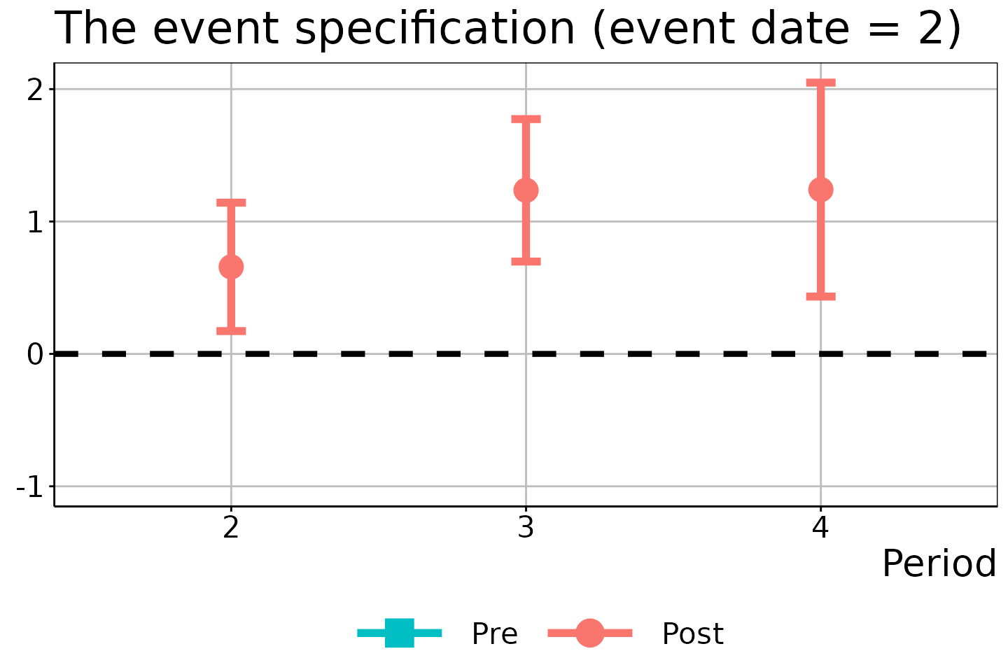

# Event date = 3
did_est$figure$e3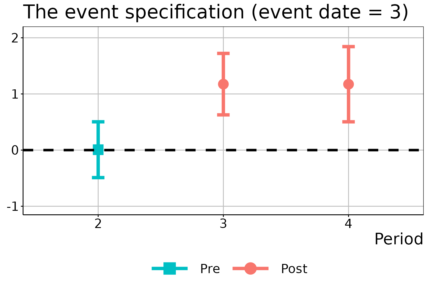

# Event date = 4
did_est$figure$e4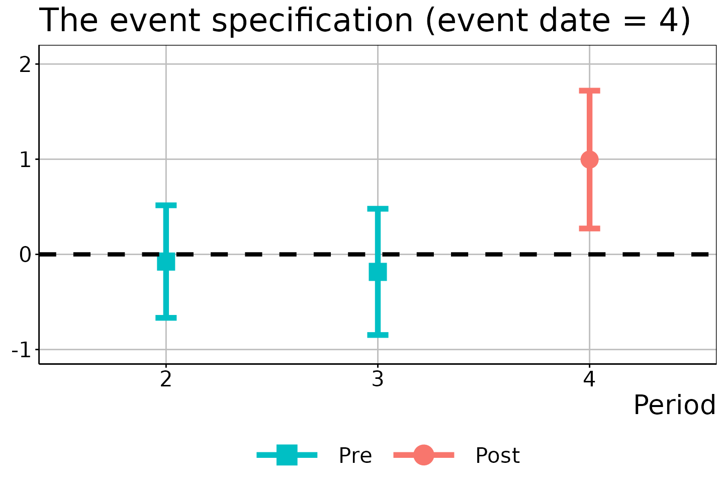

In these figures, the circles/squares and bars correspond to the ATEM estimates and \(1 - \alpha\) uniform confidence bands, with the x-axis indicating the time period \(t\).

The once specification

The DiD estimation using the once specification:

# DiD estimation
did_est <- didet::didet(yname = "Y",
                        dname = "D",
                        tname = "period",
                        idname = "id",
                        xformla = ~ X,
                        data = data,
                        specification = "once",
                        alp = 0.05,
                        nboot = 1000)

The ATEM estimation results are:

# DiD estimation
did_est$ATEM
#>   t s  r e       est        SE       CIL      CIU
#> 1 2 1 NA 1 0.6573026 0.1626075 0.2683060 1.046299
#> 2 3 1 NA 1 1.2173456 0.1593353 0.8361769 1.598514
#> 3 4 1 NA 1 1.1711503 0.2263077 0.6297673 1.712533

The resulting figure is:

did_est$figure$e1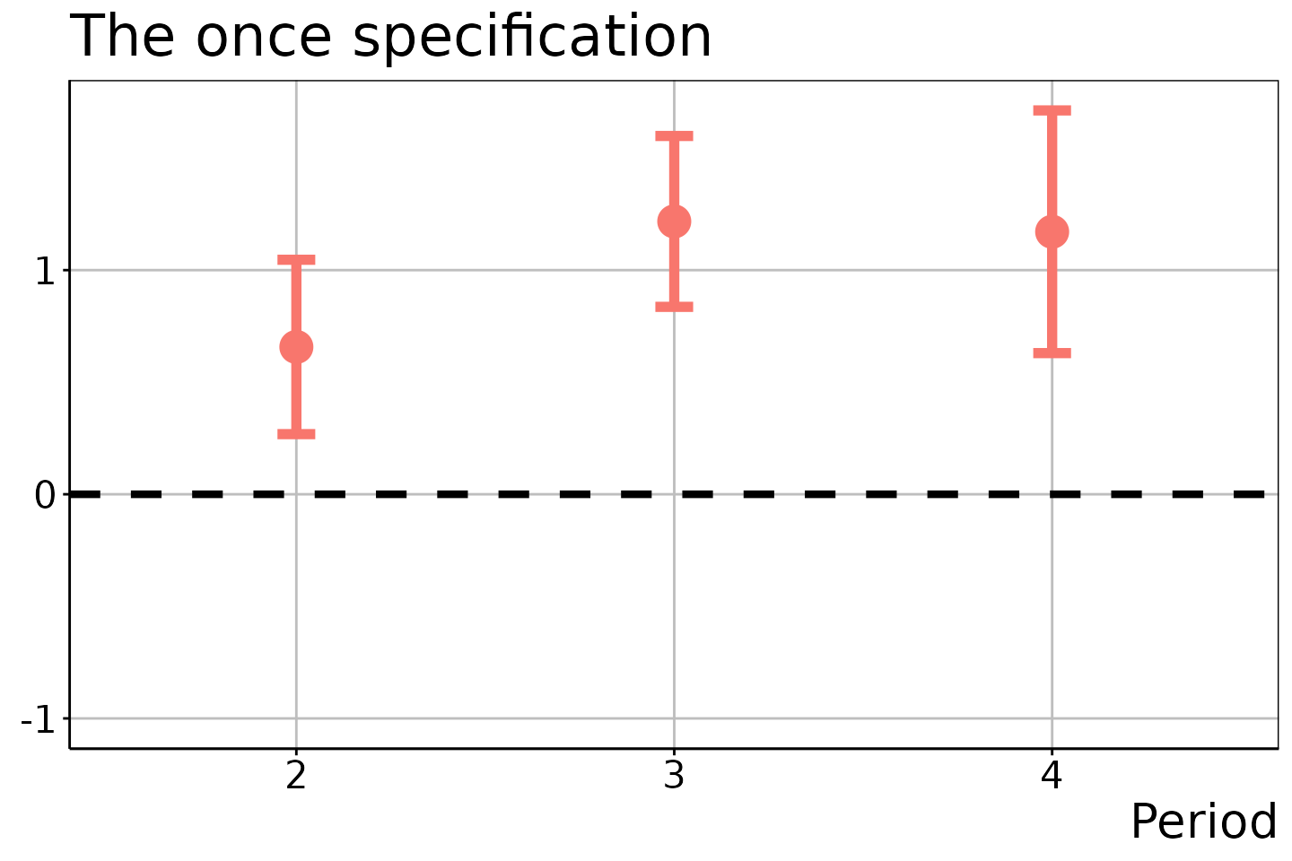

The number specification

The DiD estimation using the number specification:

# DiD estimation
did_est <- didet::didet(yname = "Y",
                        dname = "D",
                        tname = "period",
                        idname = "id",
                        xformla = ~ X,
                        data = data,
                        specification = "number",
                        alp = 0.05,
                        nboot = 1000)

The ATEM estimation results are:

# DiD estimation
did_est$ATEM
#>   t s  r e       est        SE       CIL      CIU
#> 1 2 1 NA 1 0.6573026 0.1686379 0.2142356 1.100370
#> 2 3 1 NA 1 1.1656749 0.1657341 0.7302370 1.601113
#> 3 4 1 NA 1 0.8323819 0.1951119 0.3197590 1.345005
#> 4 3 1 NA 2 1.2696071 0.2119726 0.7126857 1.826529
#> 5 4 1 NA 2 1.3969331 0.2810274 0.6585820 2.135284
#> 6 4 1 NA 3 1.1196405 0.3190303 0.2814431 1.957838

The resulting figures are:

# Number of treatment adoptions = 1
did_est$figure$e1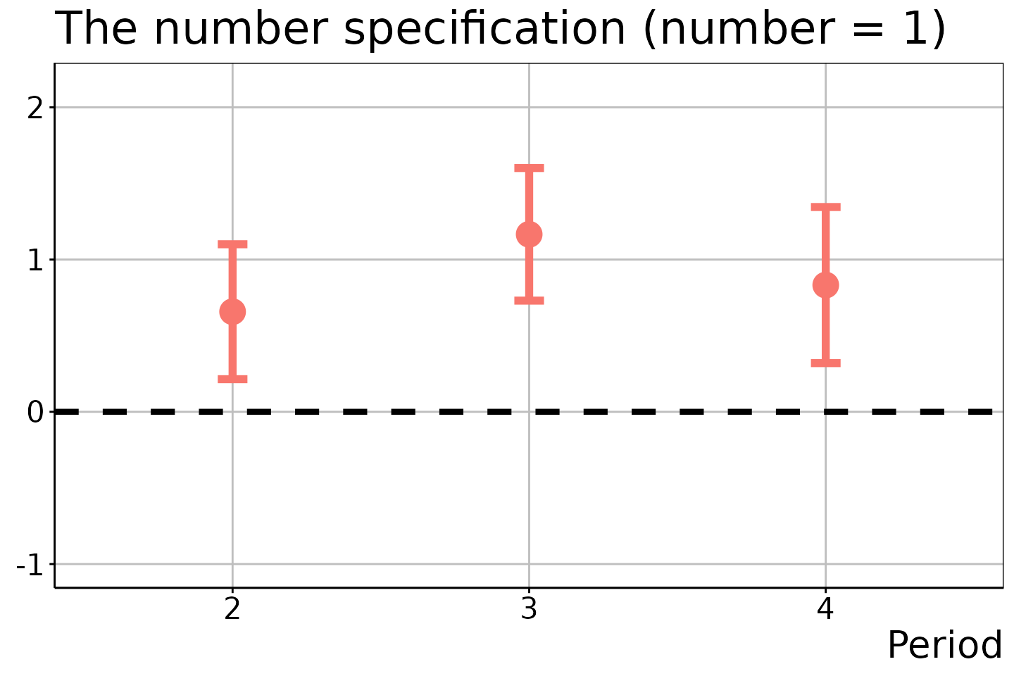

# Number of treatment adoptions = 2
did_est$figure$e2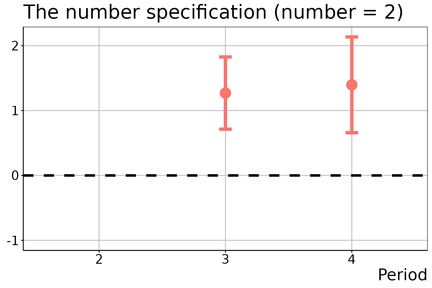

# Number of treatment adoptions = 3
did_est$figure$e3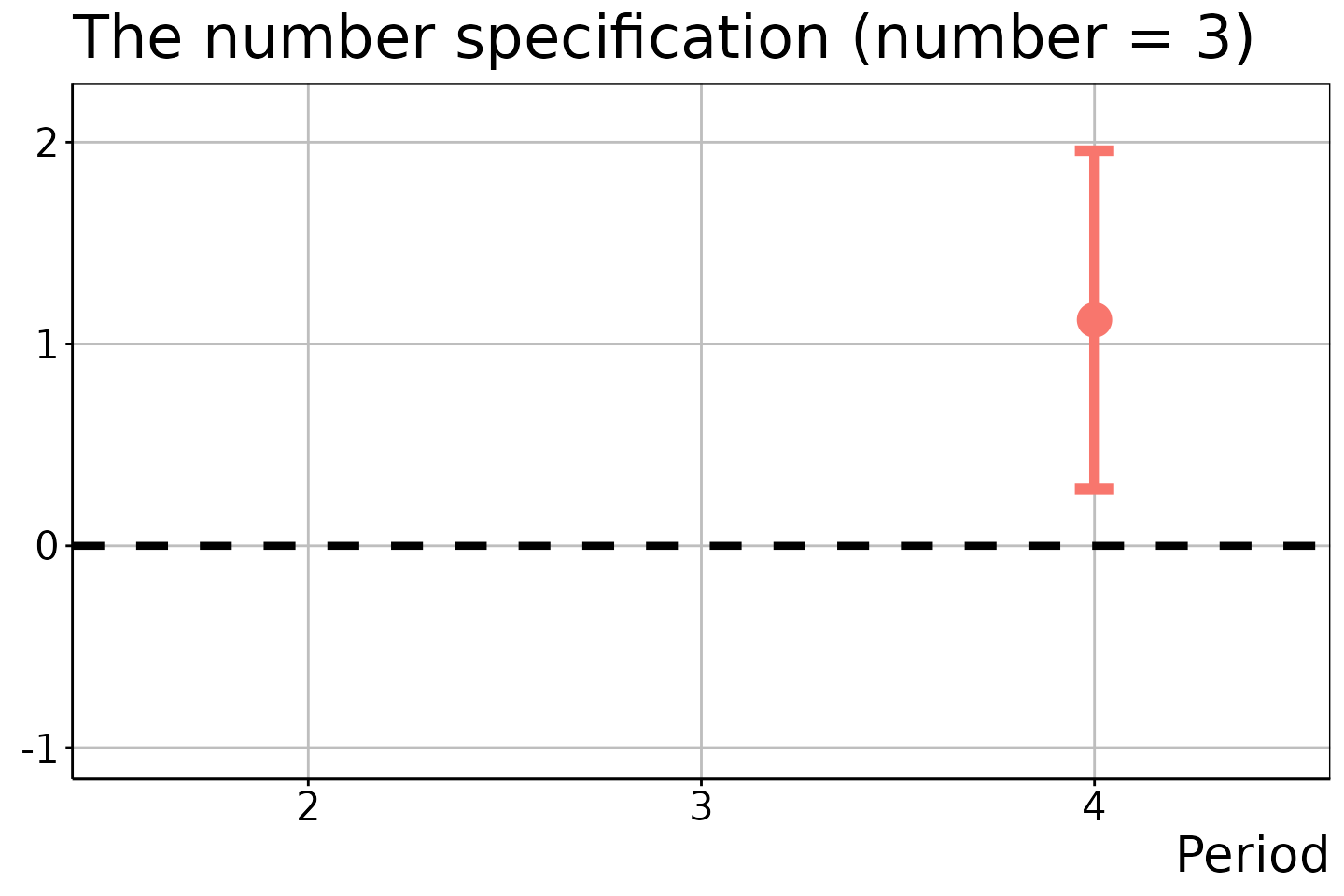

In the last two figures, the estimation results for \(t = 2\) and \(t \in \{ 2, 3 \}\) are suppressed because no units experienced the two and three times of treatment adoptions in these time periods.

Aggregation

We can obtain a single aggregation estimate by taking the time series mean of the ATEM estimates obtained from the once specification, as follows:

# DiD estimation
did_est <- didet::didet(yname = "Y",
                        dname = "D",
                        tname = "period",
                        idname = "id",
                        xformla = ~ X,
                        data = data,
                        specification = "aggregate",
                        alp = 0.05,
                        nboot = 1000)

The ATEM estimation results are:

# DiD estimation
did_est$ATEM
#>    t  s  r e      est       SE       CIL     CIU
#> 1 NA NA NA 1 1.015266 0.124448 0.7722924 1.25824

No figure is available in this case.

References

Yanagi, T., 2023. An effective treatment approach to difference-in-differences with general treatment patterns. arXiv preprint arXiv:2212.13226. Link

Takahide Yanagi (yanagi@econ.kyoto-u.ac.jp)

Introduction

Installation

Package Function

Arguments

Returns

Example

The event specification

The once specification

The number specification

Aggregation

References